
Learnings of deploying machine learning models on endpoints via ONNX

by Paul Blomstedt (Senior Data Scientist at WithSecure)
Modern approaches to securing the computing infrastructure of organisations against cyberattacks are founded on solutions that monitor all systems in a network simultaneously. This paradigm relies on endpoint sensors – lightweight programs which monitor endpoint activities and collect behavioural events that feed into detection and response systems. In this paradigm, traditional data collection approaches involve streaming all collected events into a cloud backend, where data is then processed and analysed through rules-based detection logic and machine learning models. A complementary approach to this involves placing some detection logic on the sensor itself, closer to the data source. This blog post details WithSecure’s research in TRUST aWARE into using the ONNX framework to port machine learning models and functionality onto endpoint sensors.
Before going to the question of how this is achieved, here are some of the reasons why moving intelligence to endpoints can be a good idea:
- Local context. The ability to use local endpoint-specific context may lead to better detection quality.
- Faster detection and response. Being close to the data source can enable a faster reaction time to threats, which leads to a decreased vulnerability window.
- Access to raw data. Data streamed to the backend is typically pre-processed or aggregated in some way for reasons of efficiency. Local processing can be carried out at a level of granularity, which would be infeasible in a centralised approach.
- Privacy. Local processing can enable analysis to be performed on content that cannot be upstreamed to a security backend for privacy (or confidentiality) reasons.
- Reduced volume of data transfer. With some of the analysis and detection logic moved to the endpoint, the amount of data transferred to the cloud can be reduced, making security monitoring services more affordable, especially for small organisations.
Finally, local machine learning can also be used in combination with federated learning mechanisms to share learned representations across multiple endpoints on a network (for further discussion about this approach, see the Project Blackfin whitepaper).
Benefits provided by on-sensor machine learning mechanisms must always be weighed against the downside of increasing sensor logic complexity and adversely affecting local runtime characteristics on a case-by-case basis. Most importantly, such mechanisms should have as small an impact on client machine performance as possible, while providing significant protection improvements. Later in this post, we will discuss some measures that can be taken to reduce the resource consumption of ONNX machine learning models.
Different strategies for deploying machine learning model on endpoints
Let us now examine how machine learning models can be deployed on endpoint sensors. At the moment, machine learning model development is mostly done in Python. Since we cannot assume Python runtimes are installed on all machines running our endpoint sensor (many are, for instance, Windows machines), we require a method to run trained models without the need to install a Python runtime on every endpoint. We also want a way to seamlessly integrate models into our sensors, which are binary executables usually compiled from C or C++ code. From earlier experimentation with custom low-level implementations of some of our on-sensor models we determined that, while this gave us complete control over the internals of the models, such an approach tended to lead to a lot of time spent implementing and maintaining the models, which was not always ideal.
From an implementation point of view, using existing third-party machine learning frameworks is a far more convenient approach. Some of these frameworks provide their own solutions for deploying models in different environments, not relying on Python. For example, PyTorch models can be exported and deployed using TorchScript. While this is certainly a feasible option, we would ideally like to have the flexibility of choosing the best tooling for each task without being locked into one specific framework.
ONNX and ONNX Runtime
Fortunately, there are alternatives beyond low-level customized and specialized framework-specific solutions. One of these is ONNX (Open Neural Network eXchange), which is an open format for machine learning models, supported by many of the most popular frameworks, such as PyTorch, TensorFlow, Keras, Scikit-Learn and SparkML. Models converted into ONNX format can be deployed using an ONNX Runtime, which is a high-performance, cross-platform inference engine with APIs in Python, C++, C#, C, Java, and JavaScript, among others.
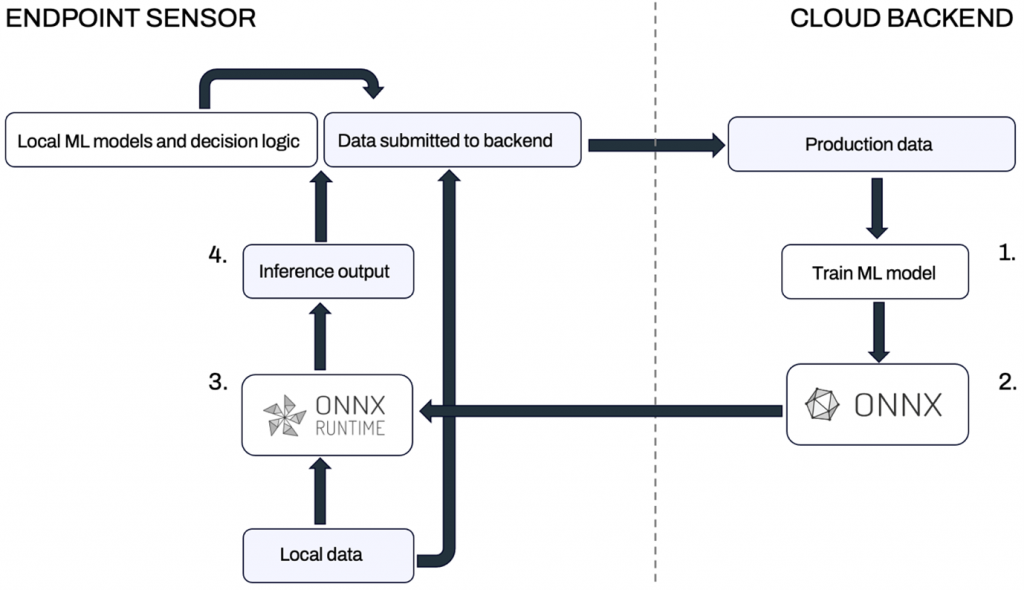
With ONNX and ONNX Runtime, the overall workflow of deploying models on endpoints is quite straightforward. The workflow, which is depicted in Figure 1, is as follows:
- Train a model in the backend using a framework which best suits the task at hand.
- Convert the model into ONNX format and send it (in an appropriately secured manner) to the endpoint.
- On the endpoint, use ONNX Runtime for inference.
- The output of the model is used as input for one or more other local ML models or directly included in data submitted to the backend.
Despite the apparent simplicity of the workflow, integrating ONNX Runtime into endpoint sensors still requires considerable effort. The good news is, however, that the ONNX technology is solid and battle-tested. Its licenses are also permissive and suitable for commercial use (Apache 2.0 for ONNX and MIT for ONNX Runtime).
In the rest of this post, we will elaborate on what we learned while experimenting with ONNX.
Preparing models for endpoints
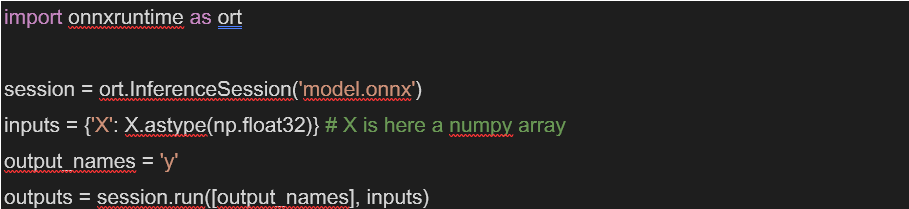
After training a model using a suitably selected machine learning framework, it must first be converted into the ONNX format. These reference tutorials give detailed examples of conversion from various frameworks. After conversion, performing some checks on the resulting model is highly recommended. ONNX has a functionality to check that a model is valid, i.e., that it has consistent input types and shapes. It is also wise to verify that the ONNX model behaves as expected, producing the same outputs as the original model. To verify an ONNX model in a continuous integration pipeline, it is possible to run inference using the ONNX Runtime Python API. To do this, first install the onnxruntime package and then load the ONNX model into an inference session.
When working with models other than deep learning models (e.g., in Scikit-Learn), it is important to note that computations are usually done with double precision (float64), while converted ONNX models use single precision (float32). In most cases, this does not cause any problems, but it is still good to keep in mind as a potential source of discrepancy between the original and ONNX models. The documentation of the sklearn-onnx package has an illustrative example about the issue.
Adding custom metadata
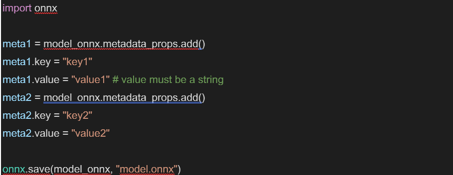
Along with the computational graph, the ONNX model also contains some additional fields such as those related to information about the converter used to produce the model. It is also possible to add custom fields as key-value pairs, which is a handy way to, for example, label models. The metadata must be set after model conversion but before saving and using the model for creating an ONNX Runtime session.
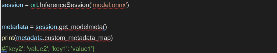
After creating a session, the custom metadata can then be accessed as follows:
Ensuring suitability for endpoints
Model size as a predictor for runtime characteristics
In the early stages of model development, optimizing predictive metrics like accuracy is often of primary concern. However, especially when deploying models in environments with strict resource constraints, such as endpoint sensors, one additionally needs to consider runtime characteristics such as latency and memory consumption. Ultimately, these characteristics need to be evaluated in the actual deployment environment, but it is important to get a rough idea of them during the development phase. When comparing alternative candidate models, we found that model size is often a simple, yet effective predictor for runtime characteristics.
With larger deep neural networks, model size itself is also of interest, and models can often be made both smaller and faster using quantisation. With traditional machine learning models, the solution often lies in finding a model type which strikes the right balance between model performance and runtime characteristics. For example, in one of our projects, we built a prototype using a random forest, which often provides a good baseline for tabular data. The predictive performance was great, and in a cloud environment we would have been quite happy with the model as it was. But when we decided to evaluate its feasibility for endpoints, it was clear that it did not meet our requirements. With some careful feature engineering and switching to a different type of ensemble, we managed to shrink the model to about 1% of its original size, with only a minor impact on predictive performance but greatly improved latency and memory consumption.
Execution time and graph optimisations
In addition to model size, another simple way of comparing candidate models or implementations is to measure the average execution time of the ONNX model with some test input. This is easily done with, for example, the Python timeit module. As an illustrative example, we conducted a simple experiment where we trained a logistic regression model with SGD on the MNIST dataset using two alternative implementations:
- A linear_model.SGDClassifier() estimator with loss=’log_loss’ using Scikit-Learn.
- A neural network with a single nn.Linear() layer and nn.CrossEntropyLoss() using PyTorch.
The size of the converted model was identical for both implementations – 32KB. This was expected, given the number of parameters is the same. The accuracy of both models was also about the same – just below 90%. However, when inference was run against the resulting ONNX models, the Scikit-Learn version had an average execution time of about 30ms, while the PyTorch model ran in 10ms, three times faster! To investigate why this was happening, we ran both models in profiling mode and inspected the resulting profile reports.
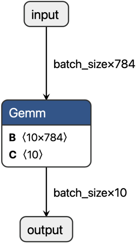
However, an even more intuitive method to understand model performance is to inspect their underlying computational graphs. This is most easily done using the Netron visualizer. Figures 2 and 3 show the graphs of the Scikit-Learn and PyTorch models, respectively. The Scikit-Learn model has a slightly more complex structure, involving computation of both the output probability and the most probable label, while the PyTorch model only has a single General Matrix Multiplication (Gemm) node, with class (log-) probabilities being implicit and baked into the loss function. This difference explains why the Scikit-Learn model takes much longer to run. If we wanted the PyTorch model to directly output probabilities, we could add a softmax layer and still have a simpler graph than with the Scikit-Learn model. While this is a very simple and slightly contrived example, it shows that it may sometimes be worth spending some time comparing implementations, and if needed, go to the trouble of writing a few extra lines of Python code to get a faster model.
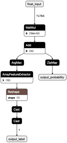
ONNX Runtime also provides graph optimisations out of the box, which can be applied to existing models. For the graph depicted in Figure 2, this type of optimization would result in the MatMul and Add operators being fused into a single Gemm operator and the two Cast nodes being reduced to one. With larger graphs this can make a substantial difference but in our small example, the effect was not too noticeable because the overall structure of the graph remained the same. Finally, some converters have different options available, which may have an impact on the resulting ONNX graph and hence the speed of inference. For example, when converting scikit-learn classifiers, it is often recommended to use options={‘zipmap’: False} to remove the ZipMap operator.
Summary
To wrap up, we conclude that there are many benefits to migrating machine learning-based detection and response logic to endpoint sensors, including the ability to work on a local context level, shorter detection and response times, access to raw data, privacy, and reduced upstream data transfer volumes. We identified ONNX as a robust and battle-tested framework that enables seamless transitioning of machine learning models developed using Python-based techniques into models that can be embedded into and run by executable binaries deployed on endpoints. Finally, as part of this study, we identified methods to ensure that resulting ONNX models function correctly and demonstrate minimal resource consumption and latency.
Acknowledgements
We’d like to thank our W/Intelligence and DRRD sensor team colleagues at WithSecure for helpful discussions. Special thanks go to Andrew Patel for the help in preparing the blog post.